Note from the future (Dec. 2020): I wrote this while working with James Bornholt on investigating some properties of a certain program synthesis algorithm, so the content in here is not really for a general audience. However, I thought it might be cool to put here in case anyone finds it and is interested in taking it futher. Keep in mind that this writeup is rough and unfinished in a few places.

Stochastic Backtracking

Spring Quarter 2019

In order to evaluate whether or not all useful lemmas are quickly learnt in the first (few) subtrees of the search space, we decided to implement a form of stochastic backtracking, which undoes decisions when a single decision has remained unchanged for too many iterations.

In particular, when a decision has remained unchanged for some $K$ iterations, we stochastically backtrack to that decision level and undo the decision. This decision is then appended to the end of the list of possible decisions for the respective partial program, to be chosen again at a later iteration. This preserves completeness almost certainly. As long as $K$ is large enough, and enough time is given, the probability of the algorithm not terminating is essentially 0. Note that $K$ can actually be dependent on other parameters, such as the corresponding decision level for the decision.

Remark. After doing some searching, this strategy may be what's known as beam stack search, or some variation of limited discrepancy beam search. The concepts are certainly similar.

Implementation

We introduce a map $\text{stoch} : \mathbb{N} \to \Delta \times \mathbb{N}$, which maps decision levels $\ell\in \mathbb{N}$ to the decision $\delta_\ell\in\Delta$ and age $t_\ell \in \mathbb{N}$. Initially, for all $\ell$ set $\text{stoch}(\ell) := \bot$. Additionally, we define some fixed $K \in \mathbb{N}$. Then, on each call to decide,

1. If $\text{stoch}(\ell_\text{cur}) = \bot$, where $\ell_\text{cur}$ is the current decision level, then set $\text{stoch}(\ell_\text{cur}) := (\delta_\text{new}, 0)$ where $\delta_\text{new}$ is the new decision made by decide. Also, for each $\ell > \ell_\text{cur}$, set $\text{stoch}(\ell) := \bot$.

2. If $\text{stoch}(\ell_\text{cur}) = (\delta_\text{old}, t_\text{old})$ and $\delta_\text{old} = \delta_\text{new}$, then do nothing. Otherwise, set $\text{stoch}(\ell_\text{cur}) := (\delta_\text{new}, 0)$, and for each $\ell > \ell_\text{cur}$ set $\text{stoch}(\ell) := \bot$.

Now, at the beginning of each synthesis iteration: for each $\ell < \ell_\text{cur}$, set $\text{stoch}(\ell) := (\delta_\ell, t_\ell + 1)$. Then (for each $\ell$), sample some random $X_\ell \sim U(0,1)$, and define $\theta_\ell = \exp(-K/(\ell + t_\ell))$. Finally, if $X_\ell < \theta_\ell$ for any $\ell$ (where in practice we choose the lowest $\ell$), backtrack to decision level $\ell$ and move $dec_\ell$ to the end of the search queue.

Evaluation

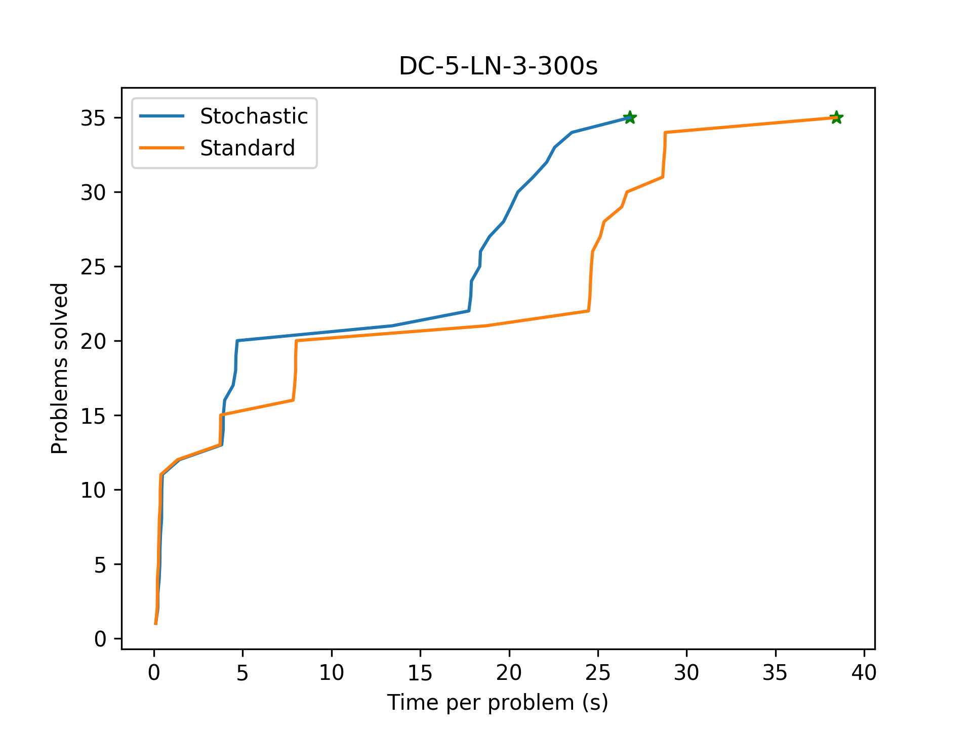
To evaluate the effect of this stochastic backtracking, we mainly wish to examine how the number of learnt lemmas changes compared to the standard synthesis algorithm. Additionally, it would help to track the strength of said lemmas as well, to understand whether or not we are simply learning more weak lemmas.

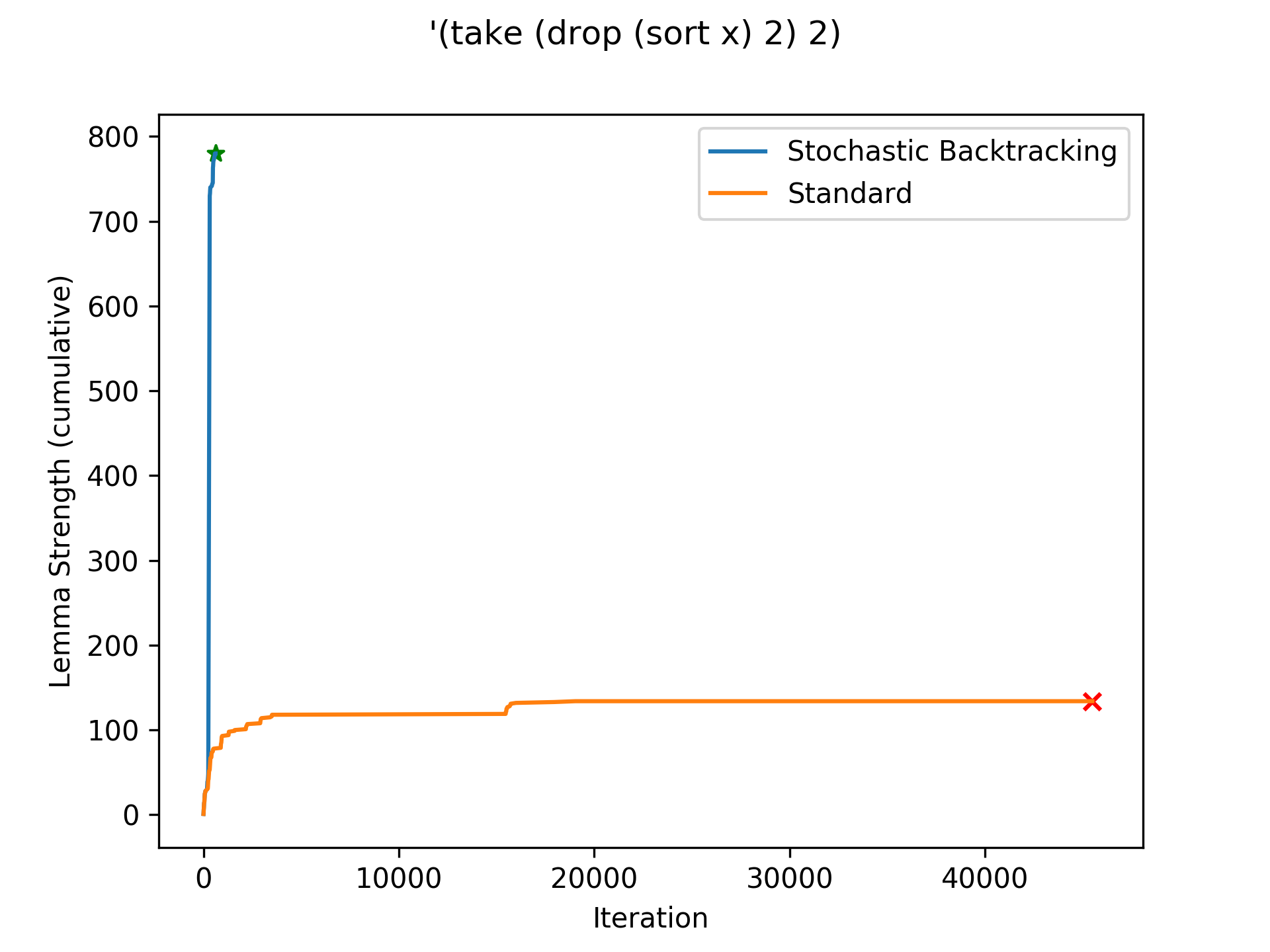
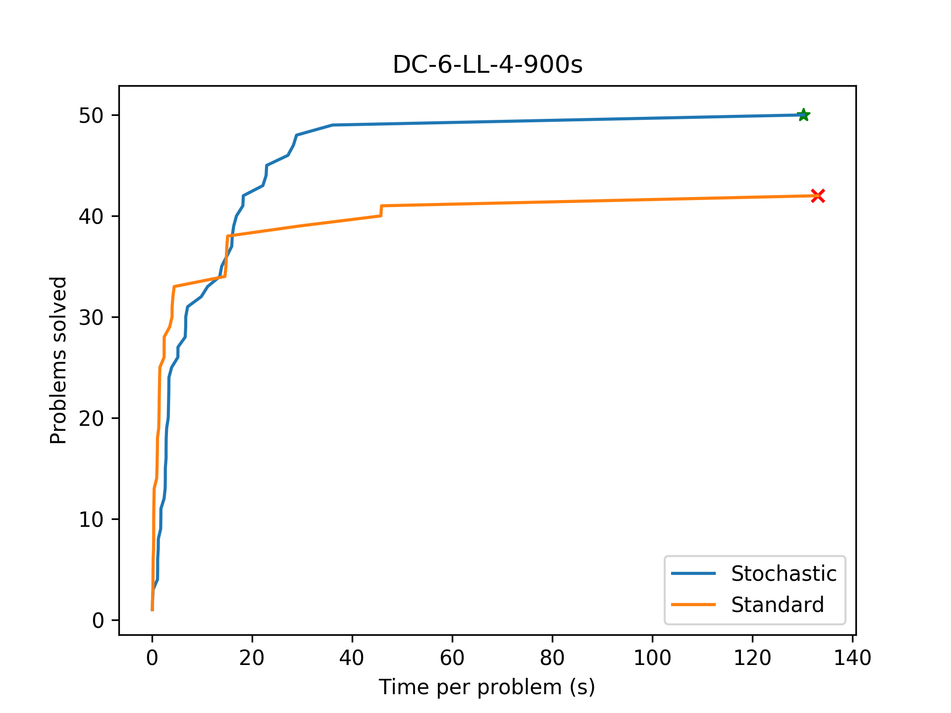
Stochastic backtracking quickly learns far more useful lemmas than the standard CDCL search, and finds the benchmark program successfully.

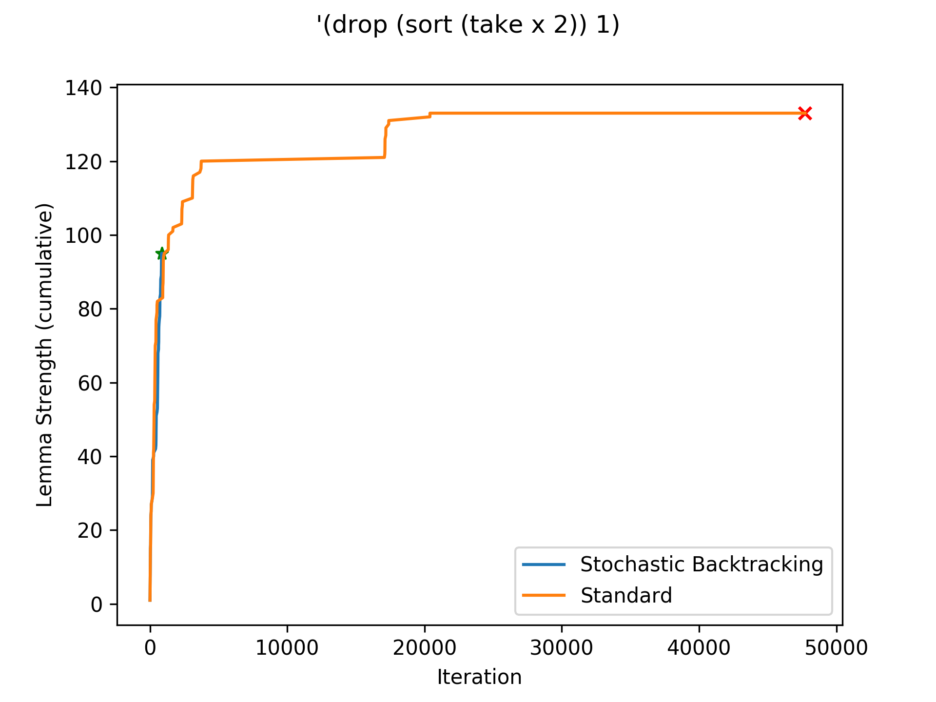
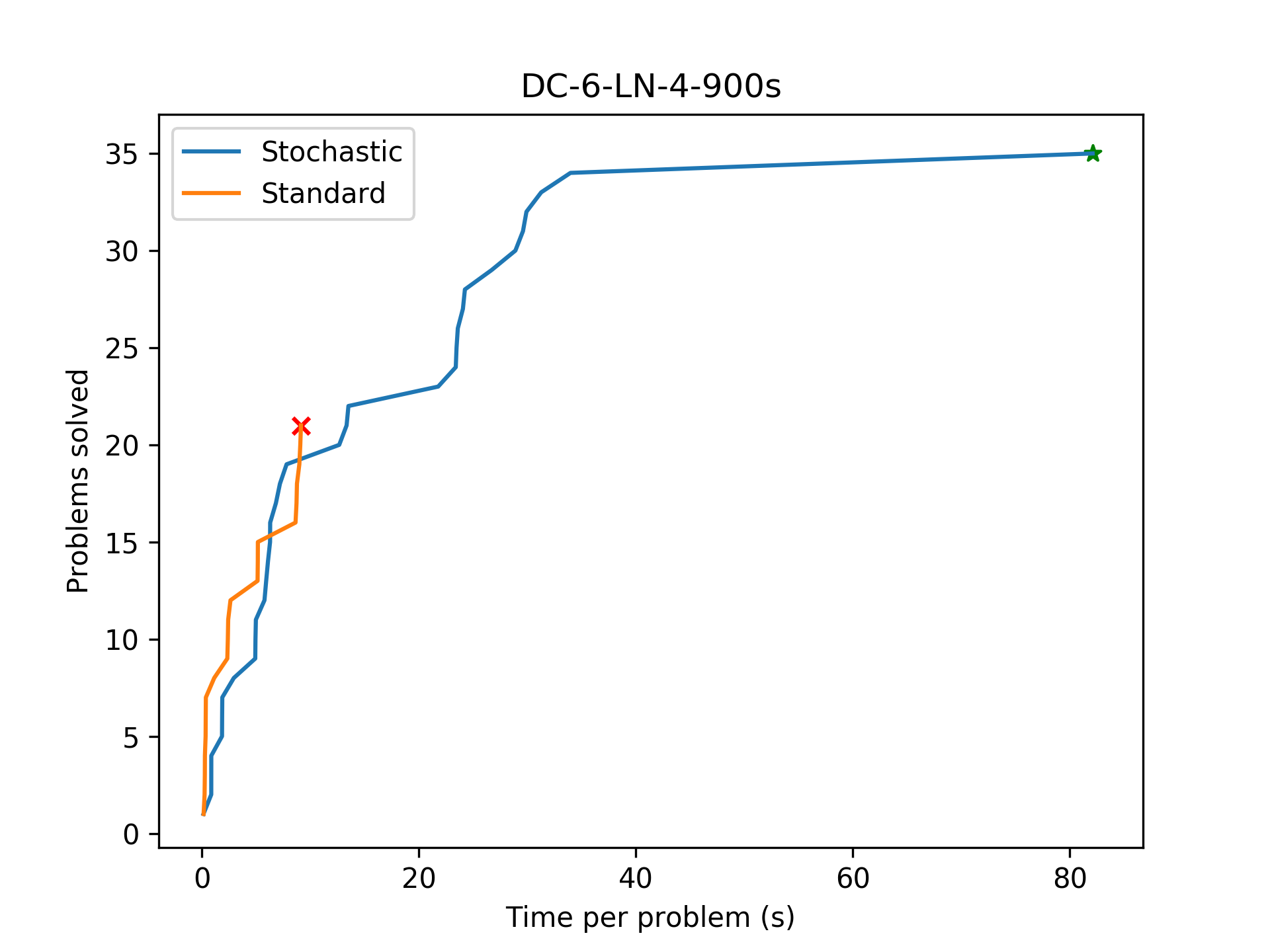
Stochastic backtracking finds the program quickly (whereas the baseline times out), but does not learn more or stronger lemmas than the baseline. In this case, stochastic backtracking likely 'guessed' the correct search subtree.

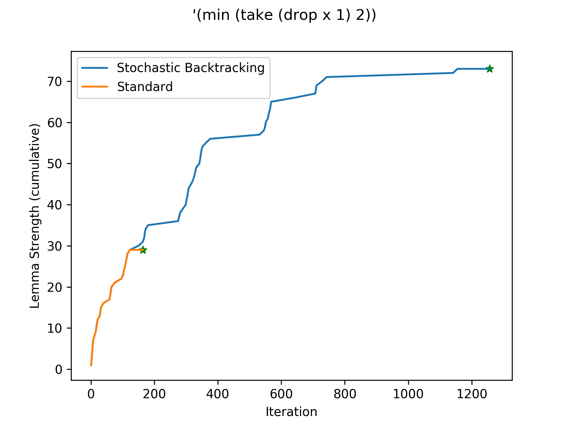
A performance regression with stochastic backtracking. In this case, stochastic backtracking mistakenly leaves the correct subtree. Due to completeness, it still finds the program eventually.

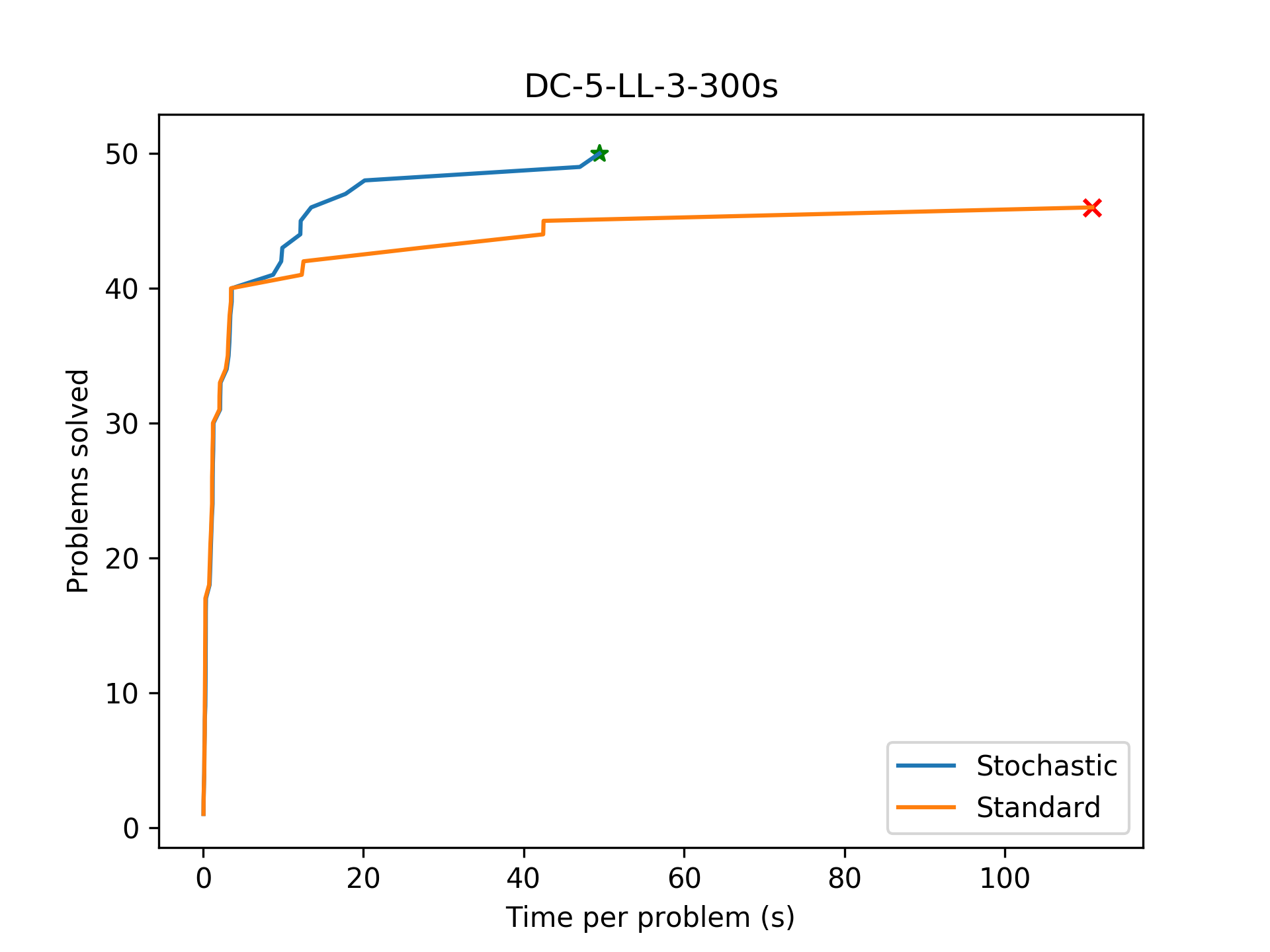
After adding stochastic backtracking, the algorithm manages to complete all benchmarks! This is a pretty major improvement.

Further Questions

At present, it is unclear if the backtracking performs well due to it being paired with conflict learning. It could be the case that this backtracking strategy is generally good (although my intuition says for deeper search trees this isn't the case). To evaluate this, we should run the stochastic backtracking algorithm with learning disabled. Additionally, to establish a further baseline, we should run a naive (but stochastic) backtracking search.

TODO: implement & run naive and no-learning stochastic algorithms.

Quantifying Lemma Strength

Winter / Spring Quarter 2019

As part of evaluating the effectiveness of the CDCL algorithm, it would be useful to have a way of quantifying the strength of the learnt lemmas. This strength should correspond to a pruning of the search space in some reasonable manner.

Counting (Partial) Programs

In order to make any meaningful measure of strength, we need to understand the size of the synthesis search space. For this we introduce some notation:

• Let $b$ denote the maximum arity of any DSL operator.

• Let $D$ denote the search depth.

• Let $H = (d, \mathcal{N})$ denote a hole at depth $d$ which can be filled by any production for the nonterminal $\mathcal{N}$. We can convert from the standard tree indexing scheme by $d= \lfloor \log_b (i + 1)\rfloor$, where $i$ is the index of the hole.

• Let $\chi_\mathcal{N}^*$ be the set of all productions for the nonterminal $\mathcal{N}$, and let $\chi_\mathcal{N}^0 \subseteq \chi_\mathcal{N}^*$ be those of null arity. Additionally, for each production $p$ of arity $k$, let $\Gamma^p$ be the $k$-tuple of nonterminals corresponding to the arguments of $p$.

Now, given a hole $H = (d, \mathcal{N})$, we wish to compute the total number of syntactically valid (concrete) programs rooted at $H$ (ignoring the rest of the tree). Denote this quantity by $C(H)$. Note that if $d = D$, then $\mathcal{N}\to \chi_\mathcal{N}^0$ since otherwise the hole would be filled with a production with further holes (which would exceed the search depth). Thus in this case, $C(H) = |\chi_\mathcal{N}^0|$. Otherwise if $d < D$, we have $\mathcal{N} \to \chi_\mathcal{N}^*$ in full. For each choice of production $p \in \chi_\mathcal{N}^*$, we then have $|\Gamma^p|$ child holes. Specifically, we have the set $\mathcal{H}_p = \{(d+1, \gamma) : \gamma \in \Gamma^p\}.$ Since our choices of $p$ filling $H$ are mutually exclusive, this is combinatorially a sum. But the productions filling the child holes are independent, so this is a product. Together, we get the following expression:

$$C(H) = \sum_{p \in \chi_\mathcal{N}^*} \prod_{h \in \mathcal{H}_p} C(h).$$

In fact, if we define $$\chi_\mathcal{N}^d = \begin{cases}\chi_\mathcal{N}^* &\quad \text{if}~d < D,\\\chi_\mathcal{N}^0&\quad\text{if}~d=D,\end{cases}$$ then $C(H) = \sum_{p \in \chi_\mathcal{N}^d} \prod_{h \in \mathcal{H}_p} C(h)$ precisely (where the product over the empty set is 1).

As we will see later, it will be convenient to define $C$ for a hole that has been filled with a production (but whose children have not been). Let $H = (d,\mathcal{N})$ as before, but this time let $p$ be the production filling $H$. Using the previous equation, we can simply define

$$C_p(H) = \prod_{h\in\mathcal{H}_p} C(h).$$

We can now easily calculate the size of the search space. With a search depth of $D$ and a root nonterminal $\mathcal{N}$, the size of the search space is given by $C((0, \mathcal{N}))$. Note that $C(H)$ is easily memoized.

Partial Programs

Call a partial program $P$ rooted iff every non-root node in $P$ has a parent node in $P$, where the root node has index $0$. Note that this implies $P$ contains the root node, or is the single root hole. From here on, we will omit the rooted qualifier and simply call such $P$'s partial programs.

Given a partial program $P$, a completion $Q$ is a concrete program satisfying $P\overset{*}{\implies}Q$ (in particular, $\text{nodes}(P)\subseteq\text{nodes}(Q)$). We can then ask the natural question: what is the cardinality of the set $\overline{P} = \{Q\mid P\overset{*}{\implies} Q\}$? For (rooted) partial programs, this is easy:

$$|\overline{P}| = \prod_{h\in\text{holes}(P)} C(h).$$

Now, call a partial program $P^*$ unrooted iff there is a non-root node in $P^*$ without a parent in $P^*$. Note: it might make more sense to not call such things partial programs at all. With this, what is $|\overline{P^*}|$? We can approach this by partially completing $P^*$ to (rooted) partial programs $P$, and then summing $|\overline{P}|$ over all such $P$'s.

Let $\text{nodes}^*(P^*) \subseteq\text{nodes}(P^*)$ be the set of non-root nodes in $P^*$ without parents in $P^*$. Define a procedure $\text{unrooted-count}(P*)$ as follows: if $\text{nodes}^*(P^*) \neq \varnothing$,

1. Pick an $n^* \in \text{nodes}^*(P^*)$.

2. Let $j$ be the such that $n^*$ is the $j$th child of its parent at index $i$ (counting from 0). Enumerate all productions $p$ such that $\Gamma^p_j = \mathcal{N}$, where $\mathcal{N}$ is the nonterminal of $n^*$'s production. If $i = 0$, then further restrict $p$ to be a root nonterminal production.

3. Return the sum of $\text{unrooted-count}(P^* \cup \{(i, p)\})$ over all such $p$.

On the other hand, if $\text{nodes}^*(P^*)=\varnothing$, then $P^*$ is rooted and we return $|\overline{P^*}|$ as computed previously. This procedure terminates as on each recursive call we are adding a previously missing parent node (and since all programs are finite).

Remark. This is potentially computationally expensive; to maintain experimental integrity, we should delay the calculation of lemma strength until after the synthesis task has completed.

Lemma Structure

As described in the conflict learning paper, the synthesis algorithm's strength is in its ability to learn lemmas from incorrect (partial) programs. These lemmas should ideally then prune large parts of the search space, by encoding equivalent-modulo-conflict (EMC) programs in a boolean formula. The synthesis algorithm would then encode the current program, and check for satisfiability against the conjunction of learnt lemmas.

Omitting some details, each lemma is a disjunction of conjunctions corresponding to the spurious program and EMC productions at each node (where a node is a pair $(i, p)$ of an index and a production). As an example, if a program $P$ with nodes $x,y,z,w$ was spurious with conflict $\kappa = \{x, z\}$, and $x \equiv_{\kappa} a$, $z \equiv_{\kappa} b$, then the encoding of the lemma $\omega = (P,\kappa)$ would be

$$[[\omega]] = (\neg \pi_x \land \neg \pi_a) \lor (\neg \pi_z \land \neg \pi_b).$$

Given a (partial) program $P$ with $N \leq |\text{nodes}(P)|$ conflicting nodes $n_1,\dots,n_N$ from conflict $\kappa$, each node $n_i$ corresponds to an equivalent-modulo-$\kappa$ class of nodes $[n_i]_\kappa$. Note that the set of conflicting nodes does not necessarily form a rooted partial program, since the parent nodes might not be conflicting. We can lift this to obtain the set of all (potentially unrooted) EM$\kappa$ partial programs w.r.t. $P$:

$$[P]^*_\kappa = \{\{\nu_i\}_{i=1}^N \mid \nu_i \in [n_i]_\kappa~\text{for}~1\leq i\leq N\}.$$

Thus, given $P$ and $\kappa$, the corresponding lemma $\omega$ (in isolation) rules out the set $\bigcup_{P^*\in [P]^*_\kappa} \overline{P^*}$ of concrete programs.

Measures

Given the above, the most intuitive measure of strength $\|\omega\|$ is simply $|\bigcup_{P^*\in[\omega_P]^*_{\omega_\kappa}} \overline{P^*}|$. This quantity counts precisely the number of concrete programs eliminated by the lemma. We can calculate this number algorithmically as follows:

1. Enumerate all choices of nodes from the EM$\kappa$ classes of nodes, so that each choice corresponds to an (unrooted) EM$\kappa$ partial program $P^*$.

2. Sum $\text{unrooted-count}(P^*)$ over all $P^*$.

Algebraically, we have $|\bigcup_{P^*\in[\omega_P]^*_{\omega_\kappa}} \overline{P^*}| = \sum_{P^*\in[\omega_P]^*_{\omega_\kappa}}\text{unrooted-count}(P').$

Overcounting

This measure works to precisely measure how much of the search space is pruned, if all lemmas prune mutually exclusive subsets of the search space. Otherwise, it will certainly overcount. Let $\Omega$ be the knowledgebase of lemmas, where for each $\omega\in\Omega$ we define

$$\overline{\omega} = \bigcup_{P^*\in[\omega_P]_{\omega_\kappa}^*} \overline{P^*}$$

as shorthand for the space of programs pruned by $\omega$. By the principle of inclusion-exclusion, the true count of concrete programs pruned is given by

$$\left|\overline{\Omega}\right| = \left|\bigcup_{\omega \in \Omega} \overline{\omega}\right| = \sum_{\varnothing\neq \Gamma\subseteq \Omega} (-1)^{|\Gamma|-1} \left|\bigcap_{\omega\in\Gamma} \overline{\omega}\right| = \sum_{\varnothing\neq \Gamma\subseteq \Omega} (-1)^{|\Gamma|-1} \left|\bigcap_{\omega\in\Gamma} \bigcup_{P^*\in[\omega_P]_{\omega_\kappa}^*} \overline{P^*}\right|.$$

To analyze this, we define the following terminology: we say that two (unrooted) partial programs $P^*$ and $Q^*$ are mutually exclusive iff there are nodes $n_1\in P^*, n_2 \in Q^*$ such that $\text{index}(n_1) = \text{index}(n_2)$ but $\text{production}(n_1) \neq \text{production}(n_2)$.

Corollary 1. It follows immediately that $\overline{P^*}\cap\overline{Q^*} = \varnothing$ for such $P^*$ and $Q^*$. Additionally, it follows that $[\omega_P]_{\omega_\kappa}^*$ is a family of mutually exclusive partial programs.

Lemma 1. Let $P^*$ and $Q^*$ be potentially unrooted partial programs. Then, $\overline{P^*}\cap\overline{Q^*} = \overline{P^*\cup Q^*}$, where we define $\overline{P^*\cup Q^*} = \varnothing$ if $P^*$ and $Q^*$ are mutually exclusive (with the natural generalization to all finite unions).

Lemma 2. For $\varnothing\neq\Gamma\subseteq\Omega$, Let $[\Gamma]^* = \prod_{\omega\in\Gamma}[\omega_P]_{\omega_\kappa}^*$, where $\prod$ is the cartesian product. Then,

$$\bigcap_{\omega\in\Gamma} \bigcup_{P^* \in [\omega_P]_{\omega_\kappa}^*} \overline{P^*} = \bigcup_{(P^*_i) \in [\Gamma]^*} \overline{\bigcup_{i} P^*_i}.$$

Proof. Induction and Lemma 1. $\blacksquare$

Lemma 3. For every distinct $(P^*_i),(Q^*_i)\in[\Gamma]^*$, the (unrooted) partial programs $\bigcup_i P^*_i$ and $\bigcup_i Q_i^*$ are mutually exclusive.

Proof. Since $(P^*_i)$ and $(Q^*_i)$ are distinct, there is an index $j$ such that $P^*_j \neq Q^*_j$. But by the definition of $[\Gamma]^*$, we have $P^*_j,Q^*_j \in [\omega^{(j)}_P]_{\omega^{(j)}_\kappa}^*$. By Corollary 1, we conclude that $P^*_j$ and $Q^*_j$ are mutually exclusive. Since the unions over $i$ are simply adding more nodes to the partial programs, they remain mutually exclusive. $\blacksquare$

Corollary 2. $\bigcup_{(P^*_i) \in [\Gamma]^*} \overline{\bigcup_{i} P^*_i}$ is a union of disjoint sets. Thus

$$\left|\bigcup_{(P^*_i) \in [\Gamma]^*} \overline{\bigcup_{i} P^*_i}\right| = \sum_{(P^*_i)\in[\Gamma]^*} \left|\overline{\bigcup_i P_i^*}\right|.$$

Furthermore,

$$|\overline{\Omega}| = \sum_{\varnothing\neq\Gamma\subseteq\Omega} (-1)^{|\Gamma|-1} \sum_{(P^*_i)\in[\Gamma]^*} \left|\overline{\bigcup_i P^*_i}\right|.$$

The number of new programs pruned by a new lemma $\omega'$ given $\Omega$ can thus be computed by

$$\|\omega'\|_\Omega = |\overline{\Omega \cup \{\omega'\}}| - |\overline{\Omega}|.$$

This measure solves the problem of overcounting. $\blacksquare$

Remark. The time complexity of a naive implementation of this computation is likely to be poor. In particular, the outer sum iterates $2^{|\Omega|}$ times, which will make the computation completely intractable even for reasonable $\Omega$'s.

$$\overline{\Omega \cup \{\omega'\}} \setminus \overline{\Omega} = \left(\overline{\omega'} \cup \bigcup_{\omega\in\Omega}\overline{\omega}\right) \setminus \bigcup_{\omega\in\Omega} \overline{\omega}.$$

Difficulty: $\overline{\omega'} \cap \bigcup_{\omega\in\Omega}\overline{\omega} \neq \varnothing$ in general. So then what is $\overline{\omega'}\cap \bigcup_{\omega\in\Omega}\overline{\omega}$? After some algebra,

$$\overline{\omega'}\cap \bigcup_{\omega\in\Omega}\overline{\omega} = \bigcup_{\omega\in\Omega}\bigcup_{P^*\in[\omega'_P]_{\omega'_\kappa}^*}\bigcup_{Q^*\in[\omega_P]_{\omega_\kappa}^*} \overline{P^*\cup Q^*}.$$ We can then write the inner two unions as a single union over $(P^*,Q^*)\in [\omega'_P]_{\omega'_\kappa}^*\times[\omega_P]_{\omega_\kappa}^*$, where it turns out each $\overline{P^*\cup Q^*}$ is disjoint from the rest by an argument similar to the proof of Lemma 3.

Despite this, we are certainly not guaranteed that the external union over $\omega\in\Omega$ is one over disjoint sets, so this approach fizzles. There might not be a way to improve upon the time complexity, if we are restricted to set theoretic operations - we may need to directly work with the program representations without dealing with the constructed spaces of eliminated programs.

Alternatively, we can use this exact measure as a threshold for learning new lemmas - in particular, we can discard lemmas whose search space pruning is below a certain number. This could allow us to keep $\Omega$ small but useful, and presents a new heuristic for keeping useful lemmas.`

Evaluation

procedure eprogs(omega) =
  let omega_P* := map(node -> eclass(node, omega.kappa), omega.conflicts)
  return product(omega_P*)

procedure strength(Omega) =
  let s := 0
  for Gamma in powset(Omega) do
    let Gamma* := product(map(omega -> eprogs(omega)))
    for PP* in Gamma* do
      s := s + (-1)^(Gamma.length - 1) * unrooted-count(union(PP*))
  return s

TODO: implement fully and run, perhaps with limit on $|\Omega|$.

---

The following experiments have not been conducted and/or are only random thoughts.

Sensitivity to Change in Inputs

How sensitive is the synthesis algorithm with respect to perturbations in the IO examples? To evaluate, run synthesis on same benchmark but sample different (valid) inputs for each run.

CDCL

Given that the main selling point of this algorithm is its ability to learn from spurious (partial) programs, it is imperative to measure the improvement over a baseline backtracking search. In particular, we want to compare the number of iterations, and for practical purposes the time taken. We will compare the following synthesis algorithms:

1. Naive backtracking search. I.e., make decisions until the program is concrete, then run on input/output examples to check correctness. If incorrect, remove last decision from the search space and make a new one.

2. Backtracking search with specifications. This is an augmentation of the previous algorithm, such that the specification of each (partial) program is checked for satisfiability w.r.t. the I/O specification. When UNSAT, the program is discarded immediately and we backtrack as before.

3. CDCL search. The full algorithm with lemma learning.

Evaluation

TODO: insert graphs.

More Stochasticity?

We can consider using techniques like simulated annealing. It's unclear how helpful stochastic techniques will be in general, although the stochastic backtracking experiment seems to work very well in current tests. The most important aspect, I think, is to balance stochastic search methods with sound and complete search strategies. This would mean injecting stochasticity into the search, rather than relying entirely on stochastic methods.

Parallel CDCL

Inspired by the stochastic backtracking experiment, we can consider running multiple instances of the synthesis algorithm in parallel. Then, each instance can e.g. be instantiated on a different root decision. When an instance exhausts its search subspace, it can be delegated to work on a subspace from another instance. All instances will share the same search space, so the pruning will happen in parallel.